Searching for significance in correlated variables
Business problem: A manager suspects that a given variable V2 is significantly predictive of a Y, but V2 is extremely correlated with V1, a variable already incorporated into your company’s simple linear model.
The manager wants the answer now: is V2 important or not?
Some things to consider:
-
Is it informative/safe to look at linear model coeffecients in a regression of V1 and V2 on Y?
-
What other strategies are worth considering?
-
Does running a linear model on the residuals of a first stage model help?
-
How can we measure results in terms of false postives vs. false negatives?
Setup
Let’s use the following setup to test [V1, V2] ∼ N(μ, Σ)
With cov(V1, V2) = .9, var(V1) = var(V2) = 1
Let V3 ∼ N(V2, .5)
Y ∼ N(V1 + V2, 1)
Approach:
We test both under the null hypothesis that V2 contains no additional information (V2nul**l) and the alternative hypothesis in which V2 does contain information (V2alt)
We simulate data using the mathematical setup described above.
library(MASS)
library(magrittr)
library(dplyr)
set.seed(5000)

createSigma <- function(corr=.9) {
Sigma <- diag(4)
Sigma[1,2] = Sigma[2,1] = corr
return(Sigma)
}

simulateData <- function(V2coef=1,corr=.9,n=20) {
  mvrnorm(n = n, mu=rep(0,4), createSigma(corr), tol = 1e-6, empirical = FALSE, EISPACK = FALSE) %>%
  as.data.frame %>%
  rename(V2_alt = V2, e1 = V3, e2 = V4) %>%
  transform(Y=  V1 + V2_alt + e1,
            V2_null = V1 + e2) %>% return
}

sampleData <- simulateData()
with(sampleData,
     plot(sampleData[c("Y","V1","V2_alt","V2_null")])
     )

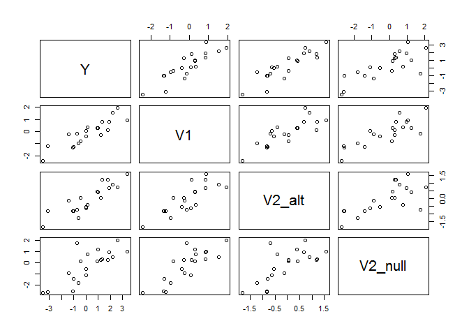
So, from the plot, we see that positive relationships between outcome Y, the standard business metric V1, as well as between Y and the new business metric V2, in both cases.
The main takeaway from this graph should be that Y vs V2alt* and *Y* vs *V*2*n**ull* look similar, even though *V*2*n**ull* has no relationship on *Y* when controlling for *V*1, while *V*2*a**lt does.
If you were to run a linear model on a model with all of these variables, you might be surprised to note that
simulation <- list(data = sampleData)
simulation$results <- with(simulation$data, list(
  fullModel = lm(Y ~ V1 + V2_alt +V2_null),
  v1Model = lm(Y ~ V1),
  v2_alt_Model = lm(Y ~ V1 + V2_alt),
  v2_null_Model = lm(Y ~ V1 + V2_null)))

#to do lapply(simulation$results, function(x) {assign(names(x)) = x})
attach(simulation$results) #just for this demo
summary(fullModel)$coef

##              Estimate Std. Error   t value   Pr(>|t|)
## (Intercept) 0.3592781  0.1689855 2.1260884 0.04941089
## V1          0.6044075  0.3548356 1.7033451 0.10784533
## V2_alt      0.9538173  0.3316292 2.8761561 0.01097033
## V2_null     0.1791071  0.2109676 0.8489793 0.40841601
So, the new variable V2 is significant but your old variable V1 no longer is…
My first answer recommendation would be to use ANOVA:
anova(fullModel)

## Analysis of Variance Table
##
## Response: Y
##           Df Sum Sq Mean Sq F value    Pr(>F)
## V1         1 46.195  46.195 83.1396 9.767e-08 ***
## V2_alt     1  4.901   4.901  8.8208  0.009027 **
## V2_null    1  0.400   0.400  0.7208  0.408416
## Residuals 16  8.890   0.556
## ---
## Signif. codes:  0 '***' 0.001 '**' 0.01 '*' 0.05 '.' 0.1 ' ' 1

anova(v1Model,v2_alt_Model)

## Analysis of Variance Table
##
## Model 1: Y ~ V1
## Model 2: Y ~ V1 + V2_alt
##   Res.Df     RSS Df Sum of Sq      F   Pr(>F)
## 1     18 14.1918
## 2     17  9.2907  1    4.9011 8.9681 0.008147 **
## ---
## Signif. codes:  0 '***' 0.001 '**' 0.01 '*' 0.05 '.' 0.1 ' ' 1
Note that Sum of Squares are the same as the first comparison in anova(fullModel), but degrees of freedom are different. That’s why anova(model1,model2) is best.
anova(v1Model,v2_null_Model)

## Analysis of Variance Table
##
## Model 1: Y ~ V1
## Model 2: Y ~ V1 + V2_null
##   Res.Df    RSS Df Sum of Sq     F Pr(>F)
## 1     18 14.192
## 2     17 13.486  1   0.70526 0.889  0.359
Someone I talked to suggested first regressing Y on V1, and then the residuals on V2.
v2_alt_ResidModel <- lm(resid(v1Model) ~ sampleData$V2_alt - 1)
summary(v2_alt_ResidModel)$coef

##                    Estimate Std. Error  t value Pr(>|t|)
## sampleData$V2_alt 0.3193023  0.2057836 1.551641 0.137246

v2_null_ResidModel <- lm(resid(v1Model) ~ sampleData$V2_null -1 )
summary(v2_null_ResidModel)$coef

##                      Estimate Std. Error   t value  Pr(>|t|)
## sampleData$V2_null 0.07502617  0.1360327 0.5515304 0.5876987
I wouldn’t recommend this approach!
Followup Questions
-
looking at linear model coeffecients and p-values is safe/not safe (pick one)
-
ANOVA is better/not better
-
We could compare procedures by using what metrics?
Investigation through Simulation
The following code builds a framework to simulate datasets and test different decision criteria with custom loss functions.
singleSimulation <- function(corr,true_effect,n_obs) {
#input: corr: number s.t. 0 < corr< 1, true_effect any number, n_obs any integer > 0
#output: a list with two linear models
data <- simulateData(V2coef = true_effect,corr = corr,n=n_obs)
res <- list()
res$model_null <- lm(Y~V1 + V2_null,data=data)
res$model_alt <- lm(Y~V1 + V2_alt,data=data)
return(res)
}

returnCoeffecients <- function(linear_model) {
  #input: a single linear model
  #output: coeffecients of V2_alt and V2_null
  linear_model$coef[3] %>% #[c("V2_alt","V2_null")] %>% // only return one??
    return
}

returnPValue <- function(linear_model) {
  #input: a single linear model
  #output: the p-value of coeffecient of 3rd variable
  temp <- linear_model %>% summary %>% `$`(coef) %>% `[`(3,4)
  #print(linear_model)
  return(temp)
}

testMethod <- function(significantMethod=returnCoeffecients,
  corr=seq(0,.95,by=.05),true_effect=(1:10), n_obs=20,n_sim=50) {
  #input: significantMethod function
  #corr: numeric vector correlation of the two variables
  #true_effect: numeric vector of true effects to measure.
  #for each combination of parameters (creates a matrix of all possible parameters)
  #and the false positive result
  true_effect <- c(true_effect) #test type II error as well!
  sim_results <- expand.grid(corr=corr,true_effect=true_effect,n_obs=n_obs,n_sim=1:n_sim)
  sim_results[paste0("sim_",1:n_sim)] <- NA
  #now, you can run these simulations however you want
  #generate data
  apply(sim_results[c("corr","true_effect","n_obs","n_sim")],1,
        function(x) {
          c(
            x["corr"],
            x["true_effect"],
            x["n_obs"],
            x["n_sim"],
            singleSimulation(corr=x["corr"],
                true_effect=x["true_effect"],
                n_obs = x["n_obs"]) %>%
            sapply(.,significantMethod)
            ) %>%
          #pull coef of interest from both regressions
          return
        }
      ) %>%
    t %>%
    as.data.frame %>%
    return
}

res<-testMethod(significantMethod=returnPValue)
save(res,file="res.RData")

euclideanDistance <- function(x,y) {
  # sample loss function
  return(sqrt(sum((x-y)^2)))
}

binaryClassification <- function(model_null,model_alt) {
  # sample loss function
  (model_null < .05) + (model_alt > .05) %>% `/`(2) %>%
  return
  }


createHeatMap <- function(df,lossFunction=binaryClassification,only_n_obs=20) {
  library(gplots)
  library(tidyr)
  # input: testMethod-result dataframe
  # output: summary data frame
  # side effect: print out a heatmap with loss function
  names(df) <- c("corr","true_effect","n_obs","n_sim","model_null","model_alt")
  temp <-
  df %>%
    mutate(true_null=0) %>%
    mutate(loss = lossFunction(model_null,model_alt))  %>%
     group_by(corr,true_effect,n_obs) %>%
    mutate(true_null = 0) %>%
    summarise(errorRate = sum(loss)/n())
  return(temp)

}

sim_res <- createHeatMap(res,lossFunction=binaryClassification)
# head(sim_res)
save(sim_res,file="heatmap.RData")
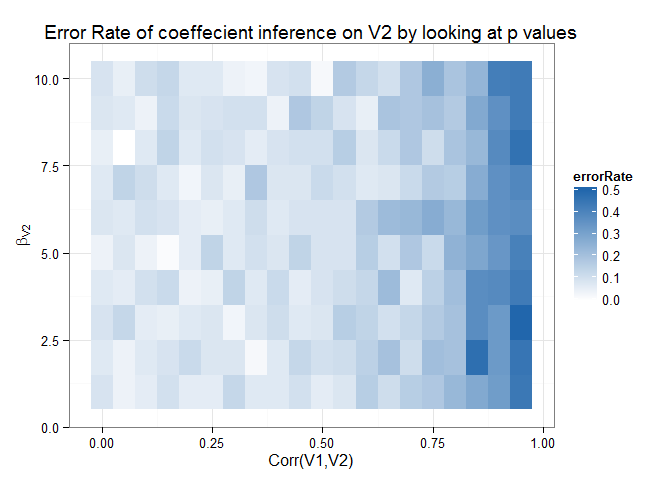
Finally, we put everything together into a heatmap that visualizes our error metric in terms of the correlation between V1 and V2, and the true value of V2.
In this example, the error rate is the false positive rate + false negative rate. Higher values are bad.
Lesson: be careful with correlated regressors!
Possible solutions:
- PCA
-
ANOVA (if you only care about is a variable significant or not)
library(ggplot2) ggplot(sim_res %>% arrange(-corr,-true_effect),aes(x=corr,y=true_effect,fill=errorRate)) + theme_bw() + geom_tile() + xlab(“Corr(V1,V2)”) + ylab(expression(beta[‘V2’])) + scale_fill_gradient2(midpoint=0, low=”#B2182B”, high=”#2166AC”) + ggtitle(“Error Rate of coeffecient inference on V2 by looking at p values”)
