Price Optimization With Adverse Selection

Estimating price elasticities is a basic step in optimizing pricing, but simply pricing based of elasticities can be a dangerous oversimplification.

In this post, I’ll show the math behind price elasticy, perform a proof of concept via simulations, and demonstrate how adverse selection can lead to losses.

Math setup:

$p$ - price, standardized for applicant risk level (i.e. risk-based pricing)

$l$ - expected loss on a sold product

$q(p)$ - Conversion, or takeup rate, of approved applicants, given price $p$

Profit per approved applicant $\pi$ is conversion rate times price (net losses):

To determine the profit-optimizing price, we distribute terms and take the derivative:

There is intuition here: A increase in price of one dollar results in:

1. An additional dollar for existing customers $q(p)$ (intensive margin)
2. Decrease in profit from forgone profit $p-l$ from lost customers $q’(p)$

The optimal pricing $p^*$ is price $p$ such that $\pi’ = 0$. Solving for $p$, we get

$p^* = \frac{q(p)}{-q’(p)} - l$

To be a maximum, the second derivative $\pi’’$ must be negative, which I leave as an exercise to the reader

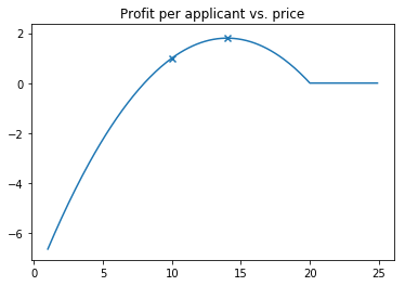
Example

For a concrete example, let’s say our company has a current price of $p=10$, average per-contract losses of $l=8$ for a loss ratio of 80%

We’ll assume that consumers have takeup rate / price elasticity of \(q(p) = max(0, 1 - p/20)\)

Taking the derivative of the profit function, we find that the company would maximize profit at $p=14$

We can plot the profit curve, with markers at current and optimal pricing

%matplotlib inline
import numpy as np
import matplotlib.pyplot as plt

START_PRICE = 10
LOSS = 8

def conversion_rate(price):
    return max(0, 1 - .05 * price)

def profit(price):
    return price - LOSS

xrange = np.arange(1, 25, step=.1)
plt.plot(xrange, [conversion_rate(p) * profit(p) for p in xrange])
price_to_plot = [10, 14]
plt.scatter(price_to_plot,[conversion_rate(p) * profit(p) for p in price_to_plot], marker='x')
plt.title('Profit per applicant vs. price')

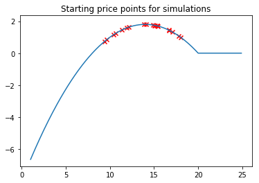
How can our company go from current pricing towards optimal pricing without knowing the takeup function?

We’ll use the following strategy:

1. Assume we start with a random price in the region where price > loss and takeup is greater than 0
2. Increase the price by 10% and observe takeup
3. Estimate elasticity of demand by computing the slope
4. Move pricing to the estimated optimal price point

And we simulate this strategy 20 times, on 2,000 applicants

np.random.seed(650)
N_SIMULATIONS = 20
starting_prices = np.random.uniform(low=LOSS+1, high=19, size=N_SIMULATIONS)
#starting_prices.sort()

plt.plot(xrange, [conversion_rate(p) * profit(p) for p in xrange])
plt.scatter(starting_prices, [conversion_rate(p) * profit(p) for p in starting_prices], c='r', marker='x')
plt.title('Starting price points for simulations')

N_APPLICANTS = 2000

new_prices = [None] * N_SIMULATIONS
takeups = [None] * N_SIMULATIONS
slope_estimate = [None] * N_SIMULATIONS
optimal_prices = [None] * N_SIMULATIONS

PRICE_EXPERIMENT_INCREASE = 1.1

for i in range(N_SIMULATIONS):
    new_prices[i] = starting_prices[i] * PRICE_EXPERIMENT_INCREASE
    takeups[i] = np.random.binomial(n=N_APPLICANTS, p=conversion_rate(new_prices[i])) / N_APPLICANTS
    slope_estimate[i] = (takeups[i] - conversion_rate(starting_prices[i])) / (new_prices[i]  - starting_prices[i])
    optimal_prices[i] = (1 - slope_estimate[i] * LOSS) / (-2 * slope_estimate[i])
    

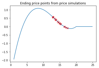
plt.plot(xrange, [conversion_rate(p) * profit(p) for p in xrange])
plt.scatter(optimal_prices, [conversion_rate(p) * profit(p) for p in optimal_prices], c='r', marker='x')
plt.title('Ending price points from price simulations')

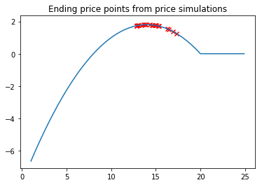
As we can see, pricing strategies is now clustered around the optimal price point.

But wait, we’re not finished

Adversarial pricing

One common problem with this approach is price-related adverse selection - that the price at which an applicant is willing to buy your product is correlated with losses. For example, a low-risk customer may purchase from a competitor offering low rates, leaving you with the subset of customers that were denied from most other providers

Here, we change the framework to incorporate price-related adverse selection by having expected losses increase as price increases:

Here’s an example where $l(p) = 3 + .05 p$

def profit(price):
    losses = 3 + .05 *price*price
    return price - losses

xrange = np.arange(1, 25, step=.1)
plt.plot(xrange, [conversion_rate(p) * profit(p) for p in xrange])
plt.title('Profit per Applicant vs. Price')

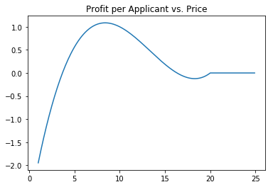
By erroneously modeling losses as independant of price, our example company raises prices higher than it should, leaving it with higher loss customers, and, in some cases, running a loss

plt.plot(xrange, [conversion_rate(p) * profit(p) for p in xrange])
plt.scatter(optimal_prices, [conversion_rate(p) * profit(p) for p in optimal_prices], c='r', marker='x')
plt.title('Ending price points from price simulations')

Even if you’re not in finance, price sensitivity may still correlate with important metrics - it’s always worth tracking CLTV of cohorts long after running a pricing experiment